Date and Time

Adithi R. Upadhya

11 August, 2022

Recap

Mutating joins, filtering joins, and set operations.

Prerequsities

library(tidyverse) 
library(lubridate)
library(nycflights13)
library(openair)

Shortcut of the day

Crtl + Shift + N


Opens a new document.

Star of the day lubridate

lubridate is an R package that makes it easier to work with dates and times.

Date/times are represented in a unique class type.

Creating date/times

There are three types of date/time data that refer to an instant in time:

  • A date. Tibbles print this as <date>.

  • A time within a day. Tibbles print this as <time>.

  • A date-time is a date plus a time: it uniquely identifies an instant in time (typically to the nearest second). Tibbles print this as <dttm>.

Today’s data nycflights13

On-time data for a random sample of flights departing New York City airports in 2013.

To get today’s time

today()
[1] "2022-08-09"
now()
[1] "2022-08-09 17:58:51 IST"

Create from a string

Helpers lubridate in automatically work out the format once you specify the order of the component.

To use them, identify the order in which year, month, and day appear in your dates, then arrange ‘y’, ‘m’, and ‘d’ in the same order.

ymd("2022-01-31")
[1] "2022-01-31"
mdy("January 31st, 2022")
[1] "2022-01-31"
dmy("31-Jan-2022")
[1] "2022-01-31"
ymd_hms("2022-01-31 20:11:59")
[1] "2022-01-31 20:11:59 UTC"

From individual date-time components

To create a date/time from this sort of input, use make_date() for dates, or make_datetime() for date-times.

new_flights <- flights %>% 
  select(year, month, day, hour, minute)

new_flights_date <- flights %>% 
  select(year, month, day, hour, minute) %>% 
  mutate(departure = make_datetime(year, month, day, hour, minute))

From other types

Sometimes we may want to switch between a date-time and a date.

Then we use as_datetime() and as_date().

as_datetime(now())
[1] "2022-08-10 07:30:54 UTC"
as_date(now())
[1] "2022-08-10"

Quiz 1

Use the appropriate lubridate function to parse each of the following dates:

d1 <- “January 1, 2010”

d2 <- “2015-Mar-07”

d3 <- “06-Jun-2017”

d4 <- c(“August 19 (2015)”, “July 1 (2015)”)

d5 <- “12/30/14” # Dec 30, 2014

Use the appropriate lubridate function to parse each of the following dates:

d1 <- mdy("January 1, 2010")

d2 <- ymd("2015-Mar-07")

d3 <- dmy("06-Jun-2017")

d4 <- mdy(c("August 19 (2015)", "July 1 (2015)"))

d5 <- mdy("12/30/14") 

Quiz 2

What happens when you parse a string which is not a valid date, like the one shown below:

ymd(c("2010-10-10", "bananas"))

What happens when you parse a string which is not a valid date, like the one shown below:

ymd(c("2010-10-10", "bananas"))
[1] "2010-10-10" NA          

Manipulating date and time

In lubridate you can get and set individual components.

Pull out individual parts of the date with the accessor functions.

datetime <- ymd_hms("2022-07-08 12:34:56")
year(datetime)
[1] 2022
month(datetime)
[1] 7
mday(datetime)
[1] 8
yday(datetime)
[1] 189
wday(datetime)
[1] 6

Date-time components

Using relevant arguments will show us the month abbreviations or full names.

Time components also extracted in the same way.

month(datetime, label = TRUE)
[1] Jul
12 Levels: Jan < Feb < Mar < Apr < May < Jun < Jul < Aug < Sep < ... < Dec
wday(datetime, label = TRUE, abbr = FALSE)
[1] Friday
7 Levels: Sunday < Monday < Tuesday < Wednesday < Thursday < ... < Saturday
hour(datetime)
[1] 12
minute(datetime)
[1] 34
second(datetime)
[1] 56

Rounding

An alternative approach to plotting individual components is to round the date to a nearby unit of time, with floor_date(), round_date(), and ceiling_date().

Each function takes a vector of dates to adjust and then the name of the unit round down (floor), round up (ceiling), or round to.

datetime <- ymd_hms("2022-07-08 12:34:56")
ceiling_date(datetime, "min")
[1] "2022-07-08 12:35:00 UTC"
floor_date(datetime, "hour")
[1] "2022-07-08 12:00:00 UTC"
round_date(datetime, "month")
[1] "2022-07-01 UTC"

Setting components

We can use each accessor function to set the components of a date/time.

(datetime <- ymd_hms("2020-07-08 12:34:56"))
[1] "2020-07-08 12:34:56 UTC"
year(datetime) <- 2022
datetime
[1] "2022-07-08 12:34:56 UTC"
month(datetime) <- 08
datetime
[1] "2022-08-08 12:34:56 UTC"
hour(datetime) <- hour(datetime) + 2
datetime
[1] "2022-08-08 14:34:56 UTC"

Or use a new function update()

(datetime <- ymd_hms("2020-07-08 12:34:56"))
[1] "2020-07-08 12:34:56 UTC"
update(datetime, year = 2020, month = 2, mday = 2, hour = 2)
[1] "2020-02-02 02:34:56 UTC"

Quiz 3

Extract month, year, and day from the data shown below, make three new columns of these. Hint use mutate(). You will have to install package called openair and then load it.

# install.packages("openair")
library(openair)
our_new_dataset <- openair::mydata %>% 
  head(50)

Extract month and year from the data shown below, make three new columns of these.

our_new_mutated_dataset <- our_new_dataset %>% 
  mutate(year_new_column = year(date), 
         month_new_column = month(date))

Quiz 4

Using the data frame created above our_new_mutated_dataset set the year values to 2022 instead of 1998.

  1. floor_date(our_new_mutated_dataset$date, “year”)
  2. ymd(our_new_mutated_dataset$date)
  1. year(our_new_mutated_dataset$date) <- 2022
  1. year(date) <- 2022

Time spans

  • Durations, which represent an exact number of seconds.

  • Periods, which represent human units like weeks and months.

  • Intervals, which represent a starting and ending point.

Durations

  • In R if you subtract two dates you get a difftime object.

  • A difftime class object records a time span of seconds, minutes, hours, days, or weeks.

  • This ambiguity can make difftimes a little painful to work with, so lubridate provides an alternative which always uses seconds: the duration.

my_age <- today() - ymd("1995-03-27")
my_age
Time difference of 9998 days
as.duration(my_age)
[1] "863827200s (~27.37 years)"

Durations

Durations come with a bunch of convenient constructors:

dseconds(15)
[1] "15s"
dminutes(10)
[1] "600s (~10 minutes)"
dhours(c(12, 24))
[1] "43200s (~12 hours)" "86400s (~1 days)"  
ddays(0:5)
[1] "0s"                "86400s (~1 days)"  "172800s (~2 days)"
[4] "259200s (~3 days)" "345600s (~4 days)" "432000s (~5 days)"
dweeks(3)
[1] "1814400s (~3 weeks)"
dyears(1)
[1] "31557600s (~1 years)"

Airthmetic with Durations

2 * dyears(1)
[1] "63115200s (~2 years)"
dyears(1) + dweeks(12) + dhours(15)
[1] "38869200s (~1.23 years)"
today() + ddays(1)
[1] "2022-08-11"
today() - dyears(1)
[1] "2021-08-09 18:00:00 UTC"

Periods

Periods are time spans but don’t have a fixed length in seconds, instead they work with “human” times, like days and months.

one_pm <- ymd_hms("2022-04-12 13:00:00", tz = "America/New_York")
one_pm + ddays(1)
[1] "2022-04-13 13:00:00 EDT"

Manipulate Periods

Periods come with a bunch of convenient constructors:

seconds(15)
[1] "15S"
hours(c(12, 24))
[1] "12H 0M 0S" "24H 0M 0S"
days(7)
[1] "7d 0H 0M 0S"
months(1:6)
[1] "1m 0d 0H 0M 0S" "2m 0d 0H 0M 0S" "3m 0d 0H 0M 0S" "4m 0d 0H 0M 0S"
[5] "5m 0d 0H 0M 0S" "6m 0d 0H 0M 0S"
weeks(3)
[1] "21d 0H 0M 0S"

Airthmetic with Periods

10 * (months(6) + days(1))
[1] "60m 10d 0H 0M 0S"
ymd("2020-01-01") + dyears(1)
[1] "2020-12-31 06:00:00 UTC"

Intervals

An interval is a duration with a starting point: that makes it precise so you can determine exactly how long it is.

next_year <- today() + years(1)
(today() %--% next_year) / ddays(1)
[1] 365

What to use??

Pick the simplest data structure that solves your problem.

If you only care about physical time, use a duration; if you need to add human times, use a period; if you need to figure out how long a span is in human units, use an interval.

Time zones

  • You can find out what R thinks your current time zone is with Sys.timezone().

  • In R, the time zone is an attribute of the date-time that only controls printing. Unless otherwise specified, lubridate always uses UTC.

Sys.timezone()
[1] "Asia/Calcutta"
head(OlsonNames())
[1] "Africa/Abidjan"     "Africa/Accra"       "Africa/Addis_Ababa"
[4] "Africa/Algiers"     "Africa/Asmara"      "Africa/Asmera"     
  • Keep the instant in time the same, and change how it’s displayed. Use this when the instant is correct, but you want a more natural display.
xa <- with_tz("2022-06-02 02:30:00", tzone = "Asia/Kolkata")
xa
[1] "2022-06-02 02:30:00 IST"
xb <- force_tz(xa, tzone = "America/New_York")
xb
[1] "2022-06-02 02:30:00 EDT"
xc <- mdy_hms("09/12/2021 09:00:10", tz = "Asia/Kolkata")
xc
[1] "2021-09-12 09:00:10 IST"

Quiz 5.1

Read two files provided in the link and name them as join_data_1 and join_data_2 accordingly. Next also look at the various statistics of these files.

Hint read_csv() and summary().

join_data_1 <- read_csv(here::here("data", "join_data1.csv"))
join_data_2 <- read_csv(here::here("data", "join_data2.csv"))


summary(join_data_1)
summary(join_data_2)

Quiz 5.2

Identify the keys in both the tables.

  1. date or Date
  1. area or Area
  1. date and area or Date and Area
  1. …1 or …1

Quiz 5.3

Convert the date column in join_data_1 and the Date column in join_data_2 to a datetime object with the timezone as “Asia/Kolkata”.

Hint ymd_hms() for date column in join_data_1 and dmy_hms() for Date column in join_data_2. Mention the timezone.

join_data_1$date <- ymd_hms(join_data_1$date, tz = "Asia/Kolkata")
join_data_2$Date <- dmy_hms(join_data_2$Date, tz = "Asia/Kolkata")

Quiz 5.4

Join the two tables (join_data_1 and join_data_2) to get a data frame called new_joined_df which contains all columns and all rows from both the tables using the key identified above.

Hint full_join().

new_joined_df <- full_join(join_data_1, join_data_2, by = c("date" = "Date", 
                                                            "area" = "Area"))

Quiz 5.5

Remove the so2 column.

new_joined_df <- new_joined_df %>% 
  select(everything(), - so2)

Quiz 5.6

Extract areas which match with “BLR”.

Hint filter().

new_joined_df <- new_joined_df %>% 
  filter(area == "BLR")

Quiz 5.7

Add a new column called ratio which is equal to pm25 / pm10.

Hint mutate().

new_joined_df <- new_joined_df %>% 
  mutate(ratio = pm25 / pm10)

Quiz 5.8

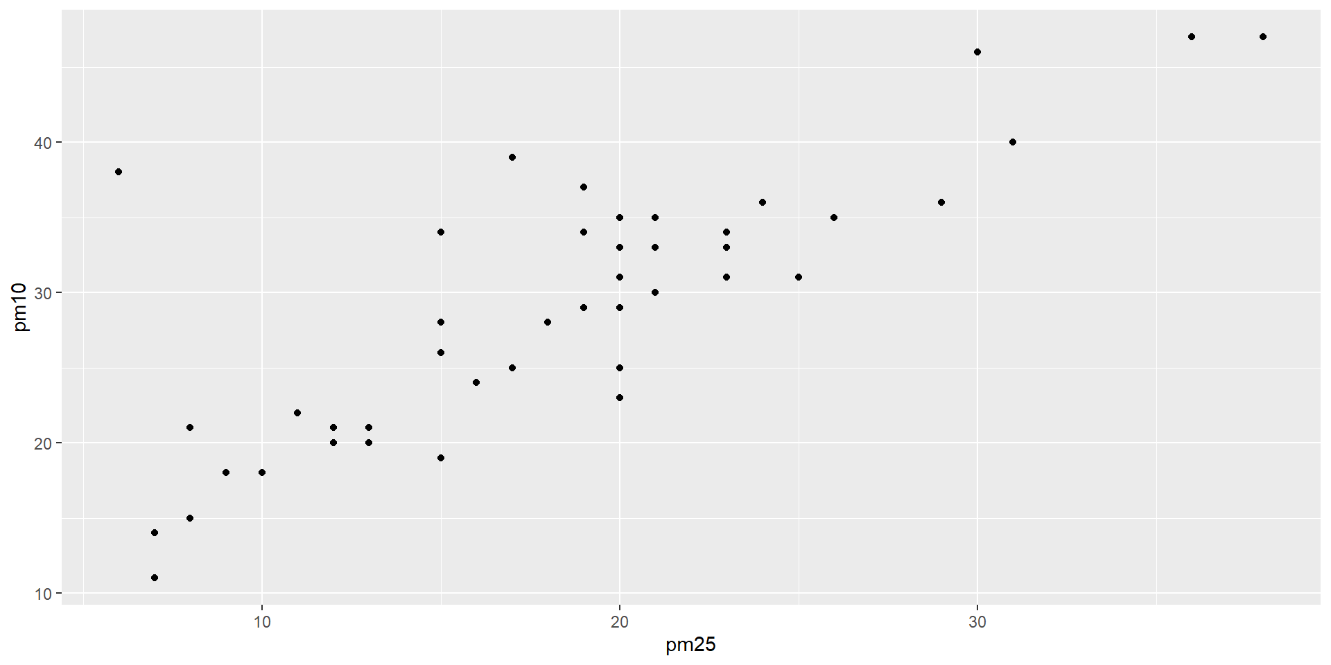
Make a scatter plot between pm25 vs pm10 using ggplot.

Hint geom_point().

 new_joined_df %>% 
  ggplot(aes(pm25, pm10)) + 
  geom_point()

Quiz 5.9

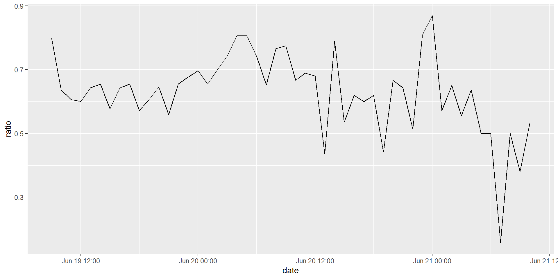
Make a time-series plot of ratio using ggplot.

Hint geom_line().

 new_joined_df %>% 
  ggplot(aes(date, ratio)) + 
  geom_line()

Resources